Multi-layer Stack Ensembles for Time Series Forecasting
A technical deep dive with a minimal implementation

Everybody knows that all models are wrong, but some are useful - a frequently omitted part is that they are wrong in different ways. It’s a handy line to throw around if you want to sound smart, but there is wisdom in it: we can exploit this error diversity. In machine learning terms, this is how ensembling works: combine the strengths of different models to get something better (sum is bigger than the parts - last cliche, I promise). Stacking goes one step further - instead of combining predictions once, it learns how to combine them.
Classification, regression, object detection - all those domain have long benefitted from sophisticated stacking. Time series did not get the love, and even in 2026 there are people who consider simple arithmetic averages as SOTA. That’s why the paper “Multi-layer Stack Ensembles for Time Series Forecasting” caught my attention:
https://arxiv.org/abs/2511.15350
Instead of searching for a single “best” model or even a single stacking strategy, the authors propose something more flexible: stack the stackers themselves. One of the reasons I really like this a lot is because it feels like a trip down memory lane: back in my Kaggle days, ensembling was the name of the game - and I have very fond memories of using hill-climbing algorithm to squeeze that one last bit of performance in the M5 competition.
In this post, I break down the core ideas behind the implementation, explains the plots generated in the notebook, and highlights why multi-layer stacking looks increasingly promising.
📓 All code lives in the companion notebook:
https://github.com/tng-konrad/time-series-lab/blob/main/mls-ensembles.ipynb
The big idea: ensembles of ensembles
Traditional forecasting ensembles combine models once - the paper argues that different stacking strategies win on different datasets, so choosing one stacker is fragile. The key insight is to stack the stackers - think of it less as one model and more as a decision pipeline:
Level 1: Base forecasting models. In this implementation, we use a mix of Seasonal Naive, Linear Regression, and Multi-layer Perceptrons (MLPs). This layes learns different views of the future.
Level 2: Stacker models that learn how to combine L1 predictions. The implementation includes a Linear Stacker (learning weighted averages) and an MLP Stacker (capturing non-linear interactions). L2 learns how those different views of the future interact.
Level 3: A final aggregator that learns how to combine the stackers themselves. We use a greedy ensemble selection algorithm - it acts as the final judge, selecting the optimal combination of L2 meta-learners to produce the final forecast. L3 learns which interaction strategy works best.
Conceptually:
data → L1 models → L2 stackers → L3 aggregator → final forecast
Combining the strengths of diverse models mitigating the risk of overfitting - but caveat emptor, it also increases the variation of the results (bias-variance tradeoff). The final can be thought of as a hierarchy of learning decisions.
Ok, let’s take it for a test drive. Before stacking anything, we need a setting where models actually disagree - otherwise stacking has nothing to learn.
Step 0: the dataset
To test the stacking framework, we need a dataset where different base models (L1) have varying performance. Stacking only shines when models disagree - if one model dominates everywhere, there’s nothing to combine.
We’ll generate a synthetic time series with diverse patterns, each composed of a unique trend, seasonality, and noise level. This heterogeneity ensures that there isn’t one “super model” at the L1 layer - instead we are setting up a scenario where a learned L2 stacker can provide value by combining the strengths of the simpler models.
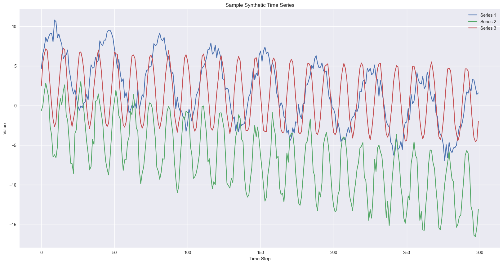
This creates a setting where:
linear models capture trend well
seasonal naive models capture the periodicity periodic data
neural networks pick up nonlinear patterns.
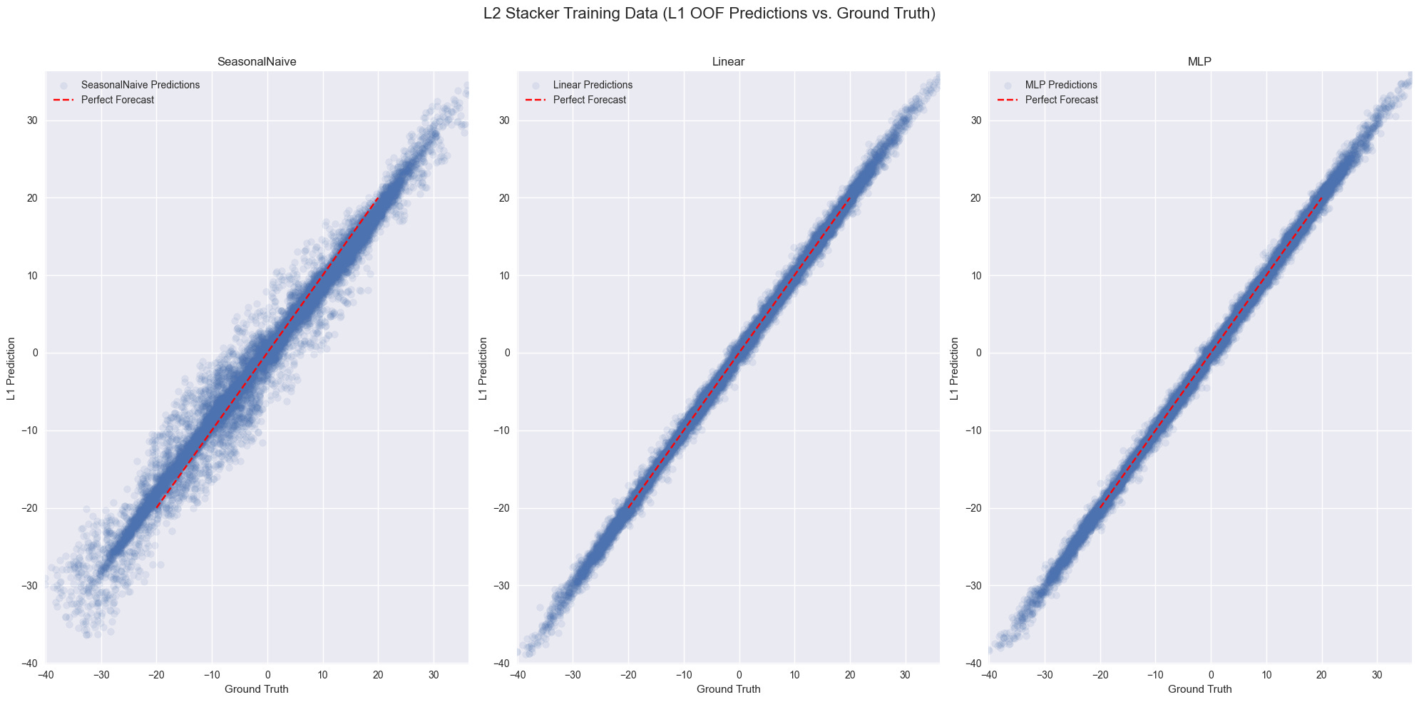
Step 1: out-of-fold predictions
The most important engineering detail is how training data for stackers is created.If you train stackers on in-sample predictions, they learn from models that have already seen the same data - which leads to leakage and overfitting. That’s why we use out-of-fold (OOF) forecasts using rolling time-series cross-validation.
Conceptually, we simulate the future multiple times - each time hiding a different slice of data - so the stacker only sees honest predictions. Here’s the core routine in pseudocode:
def generate_l1_oof_predictions(l1_models, data, num_folds, context_length, forecast_horizon):
""" Implements time series cross-validation to get out-of-fold predictions from L1 models. """
for k in range(num_folds):
# define temporal split
# train base models on past data
# predict the next window
This mirrors the training scheme described in the paper, where stackers must learn only from predictions that the base models didn’t train on. Why does it matter?
OOF predictions turn forecasting into a tabular learning problem: the stacker just learns a mapping from model outputs to the ground truth.
Step 2: learning to combine models (L2)
Once we have OOF predictions, stacking becomes straightforward. The L2 models never see the original time series - only the predictions from L1. Given several forecasts, how should we combine them? The paper implements three approaches:
MedianStacker: a strong, non-learning baseline - pointwise median of the L1 forecasts.
LinearStacker: learns weights directly from validation data.
MLPStacker: captures nonlinear interactions between models.
Stacking reduces forecasting to learning structure in model disagreements. When multiple models diverge, the stacker has signal to exploit. But here’s a twist: even stackers disagree.
Step 3: stacking the stackers (L3)
This layer operates on the predictions of the L2 stackers: we use the GreedyEnsemble selection algorithm described by Caruana et al. and use in the paper. In a nutshell, the algo train an aggregator over L2 stackers
final_prediction = L3( L2_1(L1_preds), L2_2(L1_preds), ... )
The resulting model is linear over the L2 features:s
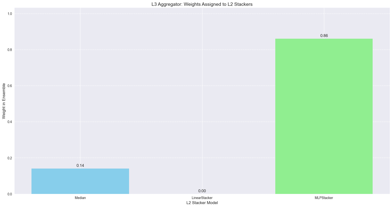
In the case of our synthetic data:
the MLP stacker dominates
but the median still receives non-zero weight.
diversity is preserved rather than eliminated.
Combining multiple stackers yields more robust performance because different learners perform best on different series.
Why It Works
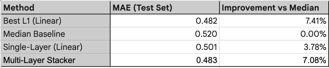
The final notebook chart compares mean absolute error across strategies.
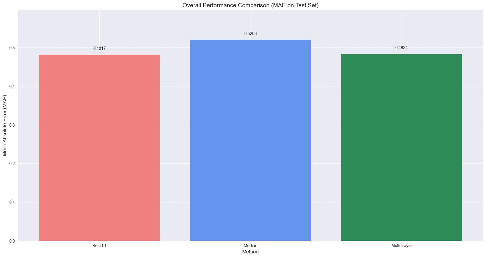
Even in this small synthetic setup, the multi-layer stack consistently improves over:
Best single model
Median averaging
Single-layer stacking
This mirrors the large-scale results reported in the paper, where multi-layer stacking achieved the highest accuracy across dozens of datasets .
Closing time
The core logic boils down to three principles:
No single forecasting model is universally best: different inductive biases capture different patterns (seasonality, trend, regime shifts)
No single stacker is universally best: linear models excel when relationships are stable; neural stackers help when interactions are complex.
A meta-ensemble solves the selection problem: instead of deciding which stacker to trust, let a higher-level learner decide dynamically.
Multi-layer stacking treats forecasting as a hierarchy of learning problems:
Learn diverse views of the future (L1)
Learn how those views interact (L2)
Learn when each interaction works best (L3)
For years, progress in forecasting has meant building bigger, better, smarter individual models. Multi-layer stacking suggests a different direction: treat forecasting as a sequence of learning decisions and not a single algorithm.
To close on a slightly philosophical note: the goal isn’t to find the perfect model, but to build a structure where imperfect ones can work together.